# Chapter 4. Waves and Interference, Schrödinger’s Cat Paradox and Bell’s Inequality
# 4.1. Waves and interference
Let us review the concept of the probability wave. The quantum wave does not carry energy, momentum or force. Its sole interpretation is that from it we can calculate the probability that a measurement will yield a particular result, e.g., that photographic film will measure a specific position of an electron in an electron beam, or that a Geiger counter will yield a specific number of gamma rays from a radioactive source. It is only during a measurement that a particle appears. Prior to the measurement, what exists is not something that can be determined by either quantum theory or by experiment, so it is a metaphysical question, not a question of physics. However, that does not mean that the metaphysical answer does not have considerable impact in both the scientific world and one’s personal world. We will say a good deal about such implications later.
Suppose we do an experiment in which machine gun bullets are fired at a wall with two holes in it (see the top panel in Figure 1). The probability P12 of finding a bullet from either hole at the backstop to the right of the wall is equal to the probability P1 of finding a bullet from hole #1 plus the probability P2 of finding a bullet from hole #2. The probability distributions are simply additive.
Figure 1
When we are dealing with waves, we have a different rule. The superposition principle is one that is obeyed by all waves in material media provided their amplitudes are not too great, and is rigorously obeyed by all electro-magnetic waves and quantum waves. It says that the net wave amplitude or height at any point in space is equal to the algebraic sum of the heights of all of the contributing waves. In the case of water waves, we can have separate waves due to the wake of a boat, the splashing of a swimmer and the force of the wind. At any point on the surface of the water, the heights of the waves add, but it is important to include the sign of the height, which can be negative as well as positive. The height of the trough of a water wave is negative while the height of a crest is positive. When a crest is added to a crest, the heights add to give a higher crest, as is shown below. When a trough is added to a crest, the heights tend to cancel. They cancel exactly if the heights of the crest and the trough are exactly equal but opposite in sign. When a trough is added to a trough, a deeper trough is created. When a crest is not lined up with either a crest or a trough, an intermediate wave is created.

Crest added to a crest gives a higher crest.

Crest added to a trough gives cancellation.

Two waves added out of phase give an intermediate wave.
See a computer animation of the superposition of two waves.
The superposition principle leads to the phenomenon of interference. The superposition, or sum, of two waves with the same wavelength at a point in space where both waves have either positive or negative heights results in a summed wave with positive or negative height greater than that of either one, as is shown below. This is called constructive interference. If the individual heights have opposite signs, the interference is destructive, and the height of the summed wave is smaller than the largest height of the two.
Looking down on a water wave. The bright lines are crests, the dark ones are troughs.

Interference of two water waves. Crests added to crests form higher crests. Troughs added to troughs form deeper troughs.
See a computer simulation of a two-slit interference pattern using water waves, using light waves and also.
An important measurable property of classical waves is power, or intensity I (power per unit area). Power is proportional to the square of the wave amplitude, and is always positive. Interference of classical waves is illustrated in the middle panel of Figure 1, where the intensity I12 at the absorber is plotted. Notice the radical difference between the graph of I>12 for the water waves and the graph of P>12 for the bullets. The difference is due to interference. Likewise, when we observe light waves, we also observe the intensity distribution, not the wave amplitude. Computer animation of the comparison between particles and waves in a two slit experiment.
For quantum waves, we already know that the property that is proportional to the square of the wave amplitude is probability. We now need to find out what interference implies for the measurement of probabilities.
Let ψ1 and ψ2 be the amplitudes, or heights, of two probability waves representing indistinguishable particles measured at the same point in space. (In quantum theory, these amplitudes are generally complex quantities. For simplicity, here we assume they are real.) The sum of these two heights is simply ψ = ψ1 + ψ2, so the probability is
ψ2 = (ψ1 + ψ2)2 = ψ12 + 2ψ1ψ2 + ψ22 (Equation 1)
This equation has a simple interpretation. The first term on the right is simply the probability that the first particle would appear if there were no interference from the second particle, and vice versa for the last term. Thus these two terms by themselves could represent the probabilities for classical particles like bullets, even though we do not ordinarily represent them by waves. If the middle term did not exist, this expression would then just represent the sum of two such classical probabilities. In the top panel of Figure 1, it would represent the probability that a bullet came through either the first hole or the second hole and appeared at a particular point on the screen. Figure 2 below shows the actual bullet impacts.
Figure 2
The middle term on the right of Equation 1 is called the interference term. This term appears only for wave phenomena (including classical waves like water waves) and is responsible for destructive or constructive interference since it can be either negative or positive. If destructive interference is complete, the middle term completely cancels the other two terms (this will happen if ψ1 = −ψ2). Because of interference, the probability distributions for waves are completely different from those for bullets. The probability distribution for electrons, labelled P12 in the bottom panel of Figure 1, has the same shape as the intensity distribution of the water waves shown in the middle panel because both distributions are derived from the square of algebraically summed wave amplitudes. The actual electron impacts are shown in Figure 3 below.
Figure 3
We can now state an important conclusion from this discussion. Whenever we observe interference, it suggests the existence of real, external, objective waves rather than merely fictitious waves that are only tools for calculating probabilities of outcomes. Consequently, in this chapter we shall assume that quantum waves are real waves and we therefore assume that the wave-function is part of external, objective reality. However, in Chapter 6 and later, we shall reëxamine this assumption and will suggest an interpretation without an objective reality.
Remember that when we detect quantum waves, we detect particles. Since we are detecting particles, it may seem that the particle must come from one hole or the other, but that is incorrect. The particles that we detect do not come from the holes, they appear at the time of detection. Prior to detection, we have only probability waves. See a computer animation of a two-slit interference pattern (Young’s experiment) that detects particles, whether photons or electrons (topic 1.1).
What happens if we try to see whether we actually have electrons to the left of the detection screen, perhaps by shining a bright light on them between the holes and the detection screen, and looking for reflected light from these electrons? If the light is intense enough to see every electron this way before it is detected at the screen, the interference pattern is obliterated, and we see only the classical particle distribution shown in the top figure. Any measurement which actually manifests electrons to the left of the screen, such as viewing them under bright light, eliminates the probability wave which originally produced the interference pattern. After that we see only particle probability wave distributions.
# 4.2. Schrödinger’s cat paradox
This thought experiment was originally created by Schrödinger in an attempt to show the possible absurdities if quantum theory were not confined to microscopic objects alone. (Since then, nobody has succeeded in showing that quantum theory actually is absurd.)
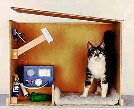

Imagine a closed box containing a single radioactive nucleus and a particle detector such as a Geiger counter (see drawing above). We assume this detector is designed to detect with certainty any particle that is emitted by the nucleus. The radioactive nucleus is microscopic and therefore can be described by quantum theory. Suppose the probability that the source will emit a particle in one minute is ½ = 50%. The period of one minute is called the half-life of the source. Animation of the radioactive decay of ‘Balonium’.
Since the wave-function of the nucleus is a solution to the Schrödinger equation and must describe all possibilities, after one minute it consists of a wave with two terms of equal amplitude, one corresponding to a nucleus with one emitted particle, and one corresponding to a nucleus with no emitted particle, both measured at the same point in space:
ψ = ψ~1~ (particle) + ψ~2~ (no particle)
where, for simplicity, we again assume the wave-functions are real rather than complex. Now, ψ12 is the probability that a measurement would show that a particle was emitted, and ψ22 is the probability that it would show that no particle was emitted. (We shall see below that the interference term 2ψ1ψ2 in ψ2 does not contribute to the final observed result.)
The remaining items in the box are all macroscopic, but because they are nothing more than collections of microscopic particles (atoms and molecules) that obey quantum theory, we assume they also obey quantum theory.
Technical note
If macroscopic objects do not obey quantum theory, we have no other theory to explain them. For example, classical physics cannot explain the following semi-macroscopic and macroscopic phenomena:
- Interference fringes (Section 4.1) have been directly produced with buckminsterfullerenes (‘buckyballs’) consisting of 60 carbon atoms and 48 fluorine atoms (C60F48).[1]
- A superconducting quantum interference device (SQUID) containing millions of electrons was made to occupy Schrödinger’s cat states.[2]
- Ferromagnetism, superconductivity and superfluidity all are quantum phenomena which occur in macroscopic systems.
- The period of inflation in the early history of the universe is thought to be quantum mechanical in origin.[3]
Hence, we assume the Geiger counter can also be described by a wave-function that is a solution to the Schrödinger equation. The combined system of nucleus and detector then must be described by a wave-function that contains two terms, one describing a nucleus and a detector that has detected a particle, and one describing a nucleus and a detector that has not detected a particle:
ψ = ψ~1~ (detected particle) + ψ~2~ (no detected particle)
Both of these terms must necessarily be present, and the resulting state ψ is a superposition of these two states. Again, ψ12 and ψ22 are the probabilities that a measurement would show either of the two states.
Put into the box a vial of poison gas and connect it to the detector so that the gas is automatically released if the detector counts a particle. Now put into the box a live cat. We assume that the poison gas and cat can also be described by the Schrödinger equation. The final wave-function contains two terms, one describing a detected particle, plus released gas and a dead cat; and one describing no detected particle, no released gas, and a live cat. Both terms must be present if quantum theory can be applied to the box’s contents. The wave-function must describe both a dead cat and a live cat:
ψ = ψ~1~ (detected particle, dead cat) + ψ~2~ (no detected particle, live cat)
After exactly one minute, you look into the box and see either a live cat or a dead one, but certainly not both! What is the explanation?
Schrödinger considered the possibility that until there is an observation, there is no cat, live or dead! There is only a wave-function. The wave-function merely tells us what possibilities will be presented to the observer when the box is opened. The observation itself manifests the reality of either a live cat or a dead cat (this is called observer created reality).
Now we must ask why the observer himself is not included in the system described by the Schrödinger equation, so we put it in the following equation:
ψ = ψ~1~ (detected particle, observer sees dead cat) + ψ~2~ (no detected particle, observer sees live cat)
If we square this expression, as in Eq. 1, we obtain
ψ^2^ = (ψ~1~ + ψ~2~)^2^ = ψ~1~^2^ + 2ψ~1~ψ~2~ + ψ~2~^2^
We know that the observer observes only a live or a dead cat, not a superposition. That means that the interference term 2ψ1ψ2 does not contribute to the observation. Why doesn’t it? Schrödinger did not have the benefit of extensive theoretical research done in the last few decades. This has shown that, because in practice it is impossible to isolate any macroscopic object from its environment, we must include its effects in this equation. Environmental effects include all of the interactions between the rest of the universe and everything in the experiment including the detector, the poison gas bottle, the cat, the box and the observer. When such effects are included and averaged over, the interference term gets averaged out, leaving only
ψ^2^ = (ψ~1~ + ψ~2~)^2^ = ψ~1~^2^ + ψ~2~^2^ (Equation 2)
Without the interference term, Equation 2 no longer describes the superposition of a dead cat and a live cat. Superficially, it is similar to the description of classical objects like bullets as was discussed above Figure 2. In the classical case, before an observation the cat is real but either alive or dead. The probabilities represent only our ignorance of the actual case. However, in the quantum case, before an observation there is no cat, live or dead. There is only a wave-function that represents the possibilities that will be manifested when an observation is made.
# 4.3. Bell’s theorem, the Aspect–Gröblacher experiments and the non-locality of reality
One of the principles considered most sacred by Einstein and indeed by most physicists up until the 1980s is the principle of local causality, or locality for short. This principle (which comes from Einstein’s theory of special relativity) states that no physical effect can be transmitted with a velocity faster than light. Also implied, but not always stated, is the principle that all physical effects must decrease as the distance between the source of the effect and the object affected increases. In practice, this principle prohibits not only all instantaneous action-at-a-distance, but also any action-at-a-distance when the distances are so large that the longest-range known force that can transmit signals, the electro-magnetic force, cannot feasibly produce the effect. If the particles of a system are assumed to be independent of each other except for physical effects that travel no faster than the velocity of light, the system is said to be local. This means, e.g., that if a measurement is made on one particle, the other particles cannot be affected before a local signal from the first particle can reach them.
In addition to locality, the other strongly held principle was the principle of objective reality (see Section 1.1). This principle states that there is a reality that exists whether or not it is observed. Prior to the discovery of quantum mechanics, this meant that this reality consisted of material particles or waves that always had definite physical properties, and which could become known either by making a measurement or by calculation using classical laws and a known initial state. For example, a particle always had a definite position and velocity prior to measurement, even though they may not have been known until a measurement or calculation was made. We call this strong objectivity. After the development of quantum mechanics, those who believe in an observer-created reality believe that only a wave-function exists prior to an observation but this is still considered to be objectively real. However, its physical parameters, such as position and velocity, are indefinite until a measurement is made. This is called weak objectivity.
Weak objectivity was difficult enough to accept by some physicists, but quantum theory predicted something else that was even harder to accept — that reality is non-local. This means that a measurement on one particle in a non-local system is correlated with a measurement on any of the other particles in the system even if no local signal passes from the first measurement to the second. For example, a measurement of the position of one particle in a non-local system is correlated with a position measurement on any of the other particles, independent of any local signals. A non-local system of particles is described by a wave-function formed by a superposition of individual particle wave-functions in such a way that all of the individual waves are locked together into a coherent whole. In such a coherent superposition, it is no longer possible to identify the individual particle components. The system behaves as a whole rather than as a collection of independent particles. We shall describe an example of a non-local system when we discuss Bell’s theorem below.
Einstein could never accept a reality which was non-local or which was indefinite. His paper written with Podolsky and Rosen in 1935 was an attempt to use a thought experiment to show that, because quantum mechanics could not describe a reality which was both local and definite, the theory was incomplete.[4]
Biographical note: This was Einstein’s last major paper on quantum theory. Until he died in 1955, he tried to devise a ‘unified field theory’ which would unite general relativity with electromagnetism in one theory. He failed in this because he could not accept the quantum description of electromagnetism. Actually, his failure is no greater than that of present-day physicists, who have produced many candidates for a unified field theory but none that can be verified with current experimental techniques.
Following the EPR paper, many physicists expended a great deal of effort in trying to devise theories that were complete, namely theories that assumed that parameters like position and velocity are at all times definite even if they are unknown, and which at the same time gave results that agree with quantum theory. (These are called hidden variable theories, which by definition assume strong objectivity.) None of these theories found general acceptance because they were inelegant, complicated and awkward to use, and the best-known version also turned out to be extremely non-local (David Bohm, see Section 6.2).
In 1964, John Bell (1928–1990, brilliant, creative Northern Ireland physicist) devised a way to determine experimentally whether reality could be described by local hidden variable theories, and derived an inequality that was valid only if local hidden variable theories were valid.[5] Furthermore, this inequality depended only on experimentally measured quantities, hence it was independent of any specific theory. Any violation of the inequality would prove that reality cannot be both strongly objective and local.
Many experiments were subsequently done to test his inequality, with the results that it was always violated, thus showing that if there is a strongly objective reality, it could not be local. In addition, the experiments always gave results that were consistent with the predictions of quantum theory. The best of these experiments were done by a group led by French physicist Alain Aspect in 1981–82.[6] These results have far-reaching implications in the interpretation of quantum theory, as we shall see below.
Note: The following discussion is somewhat technical. The reader may wish to skip directly to the bolded conclusions in this section.
The Aspect experiments used pairs of photons, the two photons of each pair being emitted in opposite directions from a calcium source. These photon pairs had the property that the polarisation directions (the vibration directions, which are always perpendicular to the propagation direction) of the two photons of a pair were always parallel to each other, but the polarisation directions of different pairs were randomly distributed.
The two sides of the experiment were 12 metres apart (see the diagram below). Each side had two detectors, to detect photons with two different polarisation directions. Each detector separately recorded an equal number of photons for all polarisation directions, showing that the photons were completely unpolarised. The detectors were wired to measure only coincidence counts, i.e., photons were recorded only if they were detected approximately simultaneously at A and B. Bell’s inequality says that, if reality is local, a certain function S of these coincidence counts, measured for all four combinations of the two polarisation angles A1, A2 and the two polarisation angles B1, B2, must be between −2.0 and +2.0. The experiments yielded a value for Sexpt of 2.70 ± 0.015. Thus Bell‘s inequality was violated.
Conclusion: The system in the first Aspect experiments was either indefinite or non-local but could not have been both definite and local. This result was independent of whether or not quantum theory was valid.
These experiments could not distinguish between a reality that is not strongly objective but is local; one that is non-local but is strongly objective; and one that is neither strongly objective nor local. Furthermore, the measured value of the function S was always in agreement with the predictions of quantum theory (SQM = 2.70 ± 0.05), which assumes that the photons are described by wave-functions.

Bell’s function F is a measure of the correlations between the polarisations (vibration directions) measured at the two sides A and B. The existence of correlations does not itself prove that reality is indefinite or non-local. In fact, correlations can exist between measurements at the two sides whether the photons are local and definite (‘real’ photons) or whether they are non-local and indefinite. If they are local and definite, correlations will exist if the two ‘real’ photons emitted by the source are individual particles that are polarised parallel (or perpendicular) to each other. If they are non-local and indefinite, correlations can exist if the system is described by a wave-function that is a coherent superposition of the waves of the two photons (an ‘entangled pair’). Because such a wave-function represents a coherent whole rather than individual particles, it permits correlations that are greater than can exist with local, definite photons. That is why S is greater for entangled photons than for local, definite photons, and why the measured violation of Bell’s inequality is consistent with photons described by quantum theory.
Next, the Aspect group showed that the violation of Bell’s inequality measured in the first experiments could not have been due to some unknown type of local signal carrying polarisation information from one set of detectors to the other, rather than being due to the properties of the wave-functions alone. By definition, such a local signal would have had to propagate with a velocity no greater than that of light. Thus, the next set of experiments was designed to prevent any possible local signal transmission between the two sides from affecting the results.[7] To do this, the decision about which polarisation direction to measure at side A was made after a possible local signal from a measurement at side B was already in transit, and similarly for the converse. Therefore, a polarisation measurement at B could not affect a polarisation measurement at A, and vice versa. The conclusion from the second set of experiments was that the correlations could not have been a result of local signal transmission. This implied that their system was non-local.
Now we must ask whether any class of hidden variable theories, which are all designed to be strongly objective, can be excluded by experiment. (Bell’s theorem and the Aspect experiments say only that hidden variable theories must be non-local. It does not exclude any class of non-local hidden variables theory.) To help answer this question, an inequality similar to Bell’s inequality was recently devised by Tony Leggett.[8] An experiment was then done by S. Gröblacher et. al. to see whether a broad class of hidden variable theories (that are all non-local) could be excluded.[9]
Gröblacher et al. concluded that no hidden variable theory that is not counterintuitive (that is not bizarre) can describe reality. If so, then reality cannot have definite properties before measurement. The Aspect and Gröblacher experiments taken together strongly imply that reality is both indefinite and non-local (there are no ‘real’ particles). This conclusion is independent of whether or not quantum theory is valid.
The experiments of Aspect and Gröblacher et al. do not prove quantum theory to be valid but are consistent with its predictions. [No number of experiments can prove that any physical theory is valid. However, it takes only one well-done experiment, if it is confirmed independently by independent researchers, to prove that a physical theory is invalid.] We have seen in Section 3.2 that, if quantum theory is valid, it does not tell us what is there before a measurement. This is the indefiniteness property. In Chapter 6 we shall also see that quantum theory is non-local.
In a non-local system, a measurement made at one end of the system is correlated with a measurement made at the other end even if no local signal passes between the two. It might be thought that, because non-local correlations can exist between events occurring at two different points, observers at these two points could use these correlations to communicate instantaneously with each other in violation of Einstein’s special theory of relativity. However, the non-locality of quantum theory implies a correlation between data sets, not a transmission of information at greater than light velocities. Thus, the special theory is not violated. We can see this by realising that the photons detected at either A or B alone occur completely randomly both in time and in polarisation. Consequently, observer A sees no information in his data alone, and likewise with observer B. It is only by later comparing these two random sets of data that a correlation between the two sets can be discovered.
Technical note
Theoretical calculations indicate that the human eye might be sensitive enough to detect the correlations from entangled pairs of photons without the aid of electronic devices.[10]
There can be strong correlations between two random sets that cannot be discovered by looking at one set alone. This is illustrated by the example of random stereograms (see Magic Eye diagrams and below) which, when first viewed, look like near-random patterns of coloured dots (see below). However, there are actually two separate near-random patterns present, and they are displaced from each other by a distance roughly equal to the spacing between a person’s eyes. Thus, by looking at the pattern with the direction of the eyes non-convergent as if looking some distance away, the two eyes see different patterns. The correlations between the patterns are discerned by the brain, and a three-dimensional image is seen.
Magic Eye images may be easier to see if viewed on paper rather than a computer screen. If possible, print this image and follow the instructions below. (You don’t need to print in colour.)
Hold the centre of the printed image right up to your nose. It should be blurry. Focus as though you are looking through the image into the distance. Very slowly move the image away from your face until the two squares above the image turn into three squares. If you see four squares, move the image farther away from your face until you see three squares. If you see one or two squares, start over!
When you clearly see three squares, hold the page still, and the hidden image will magically appear. Once you perceive the hidden image and depth, you can look around the entire 3D image. The longer you look, the clearer the illusion becomes. The farther away you hold the page, the deeper it becomes. Good Luck!
# 4.4. Another experimental violation of observer independent theory
Section 4.3 discussed conflicts between the hidden variables and quantum descriptions of experiments that were done on entangled quantum objects, such as pairs of entangled photons. Recently, measurements were done on pairs of trapped ions that were not entangled, and even with these non-entangled particles, the results were consistent with quantum theory but inconsistent with the assumption of observer-independent particles.[11]
# Footnotes
the famous EPR paper — A. Einstein, B. Podolsky and N. Rosen, Can A Quantum-Mechanical Description of Physical Reality be Considered Complete?, Phys. Rev. 47 (1935) 777–780 ↩︎
J. S. Bell, On the Einstein-Podolsky-Rosen Paradox, Physics 1 (1964) 195–199 ↩︎
Alain Aspect, Phillipe Grangier and Gérard Roger, Experimental realisation of Einstein-Podolsky-Rosen-Bohm Gedankenexperiment: A New violation of Bell’s inequalities, Phys. Rev. Lett. 49 (1982) 91–94 ↩︎
Alain Aspect, Jean Dalibard, and Gérard Roger, Experimental test of Bell’s inequalities using time-varying analysers, Phys. Rev. Lett. 49 (1982), 1804–1807 ↩︎
Non-local hidden-variable theories and quantum mechanics: An incompatibility theorem, Foundations of Physics, 33 (2003) 1469–1493 ↩︎
An experimental test of non-local realism, Nature 446 (2007) 871–875 ↩︎
Brunner, Branciard and Gisin, Possible entanglement detection with the naked eye, Phys. Rev. A 78 (2008) 052110 ↩︎
Kirchmair, Zähringer, Gerritsma, Kleinmann, Gühne Cabello, Blatt and Roos, State-independent experimental test of quantum contextuality, Nature 460 (2009), 494–497 ↩︎